

The Oracle Instructor

Pickleball & Longevity
Studien zufolge trägt die Trendsportart Pickleball in nahezu idealer Weise zur Langlebigkeit bei! Wer möchte nicht sein Leben bei guter Gesundheit um 10 Jahre verlängern? Mit Pickleball könnte das mit Freude und Spielspaß gelingen.
Copenhagen City Heart StudyEine höchst beachtenswerte Studie ist die Copenhagen City Heart Study (CCHS).
Diese Langzeitstudie hatte 8577 Teilnehmer, die über einen Zeitraum von 25 Jahren (von Oktober 1991 bis März 2017) beobachtet wurden.
Es sollte untersucht werden, welcher Zusammenhang zwischen der Ausübung bestimmter Sportarten und der Lebenserwartung besteht. Verglichen mit einer Kontrollgruppe, die keine nennenswerte sportliche Aktivität ausübte ergab sich diese Reihenfolge der Erhöhung der Lebenserwartung:

Ja, von Pickleball ist hier noch nicht die Rede. Das liegt daran, dass diese Sportart 2017 noch keine große Popularität hatte. Ich werde den Zusammenhang gleich herstellen. Was haben die ersten drei Plätze gemeinsam?
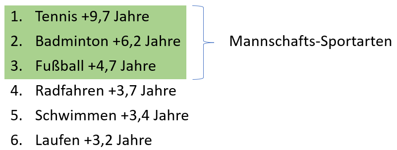
Mannschafts-Sportarten fördern die soziale Interaktion stärker als Sportarten, die auch allein betrieben werden können. Häufigere soziale Interaktion korreliert wiederum positiv mit Langlebigkeit. Platz 1 und 2 heben sich noch etwas vom dritten Platz ab. Was haben Tennis und Badminton gemeinsam?

Rückschlag-Sportarten erfordern nicht nur Kraft, Schnelligkeit und Ausdauer, sondern darüber hinaus stellen sie relativ hohe kognitive Anforderungen. Hand-Auge-Koordination ist stark gefordert, ebenso wie taktisches und situatives Verständnis und Reaktions-Schnelligkeit. Den Spitzenreiter dieser Rangfolge trennen allerdings immer noch stolze 3,5 Jahre zusätzlicher Lebenserwartung vom zweiten Platz. Woran könnte das liegen?
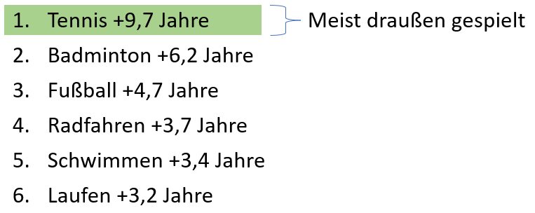
Während Badminton nahezu ausschließlich in der Halle gespielt wird, findet Tennis überwiegend auf Außenplätzen statt. Sport im Freien hat gesundheitliche Vorteile: Das wichtige Vitamin D kann dabei vom Körper hergestellt werden. Die Helligkeit ist draußen um ein Vielfaches stärker als in geschlossenen Räumen, was Depressionen vorbeugt.
Bis hierhin könnte man sagen: Glückwunsch an die Tennis-Spieler; alles richtig gemacht! Was hat das mit Pickleball zu tun? Hierzu möchte ich eine zweite große Studie anführen, die Apple Heart and Movement Study.
Apple Heart and Movement StudyDiese Studie wurde im Oktober 2023 durchgeführt und hat über 250.000 Pickleball- und Tennistrainings analysiert. Möglich war diese Analyse durch die Apple-Uhren, die dabei von den Spielern getragen wurden. Ich führe die Apple Heart and Movement Studie hier an, weil sie zeigt, dass die körperlichen Anforderungen von Tennis und Pickleball höchst ähnlich sind. Also sind auch ähnlich positive Effekte von Pickleball für die Langlebigkeit zu erwarten, zumal auch Pickleball sehr häufig draußen gespielt wird.

Die durchschnittliche Belastung beim Tennis ist etwas höher (um 9 Herzschläge pro Minute), dafür ist die durchschnittliche Dauer des Trainings beim Pickleball 9 Minuten länger. In Bezug auf soziale Interaktion steht die Pickleball-Community den Tennis-Spielern sicherlich nicht nach. Ein entscheidender Unterschied und Pluspunkt für Pickleball ist aber: Es ist erheblich leichter zu erlernen als Tennis! Das ist gerade für Menschen fortgeschrittenen Alters relevant, die zur Steigerung ihrer Gesundheit einen Rückschlag-Sport anfangen wollen.
Außerdem macht es einfach wahnsinnig viel Freude, Pickleball zu spielen! Und was man mit Freude tut, tut man öfters und regelmäßig, wie auch diese Erhebung in der Apple-Studie zeigt: Die Anzahl von Pickleball-Trainingseinheiten ist stetig gestiegen, während die Teilnahme an Tennis-Trainings starken Schwankungen unterlag.
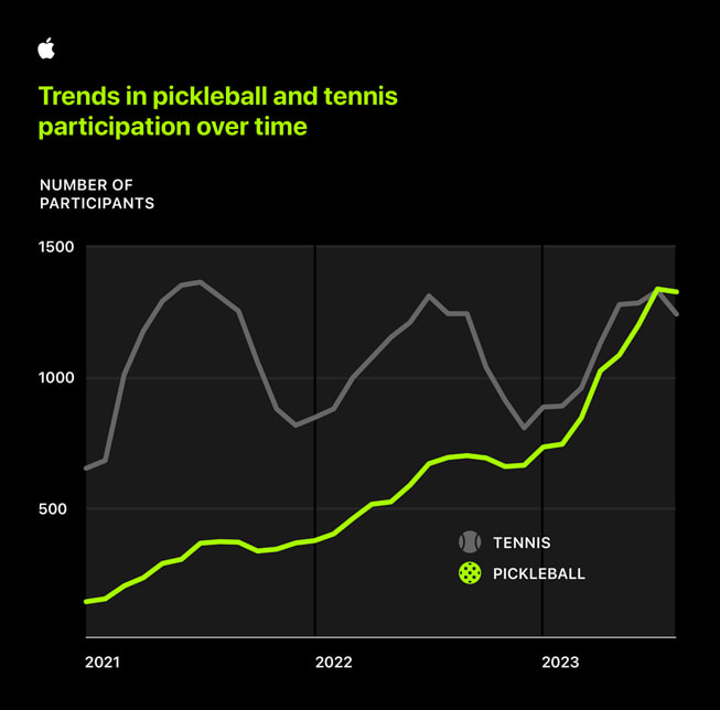
Quelle: Apple Heart and Movement Study
Zusammenfassend kann ich jedem, der an einer Verlängerung seiner Lebenserwartung durch Sport interessiert ist nur ans Herz legen, es einmal mit Pickleball zu versuchen! Pickleball spielen ist natürlich allemal besser als keinen Sport zu machen. Es scheint im Lichte der obigen Studien aber auch besser für die Langlebigkeit zu sein als manch anderer Kandidat, wie z.B. Laufen.
Pickleball spielen auf einem Badminton Feld
Ein Badminton-Spielfeld kann man sehr schnell und kostengünstig für Pickleball umwidmen. Das macht es für Sportlehrer und Sportvereine leicht, den Trendsport anzubieten.
Die Außenmaße eines Badminton-Doppelfeldes sind identisch mit den Außenmaßen eines Pickleball-Felds:

Badminton Spielfeld
Beim Pickleball gibt es übrigens keinen Unterschied in den Außenmaßen des Spielfelds bei Einzel oder Doppel. Also die Außenmaße sind schon mal gleich, da muß man gar nichts ändern. Nur die Auschlaglinie beim Badminton (in 1,98 m Entfernung vom Netz) ist nicht identisch mit der NVZ-Linie beim Pickleball:

Pickleball Spielfeld mit NVZ
Die NVZ ist in 2,13 m Abstand vom Netz. Man muß also nur jeweils eine Linie im Abstand von 15 cm von der Badminton-Aufschlaglinie aufkleben, schon hat man aus einem Badminton-Feld ein Pickleball-Feld gemacht!
Dafür eignet sich z.B. gut das Gauder Malerkrepp (ca. 12 Euro für drei Rollen); es läßt sich leicht aufkleben, hält gut und ist rückstandslos ablösbar. Hat man in 5 Minuten aufgeklebt:

Was noch fehlt ist ein Pickleball-Netz – das Badminton-Netz ist mit 1,55 m Höhe zu hoch. Ein mobiles Pickleball-Netz kostet unter 200 Euro und ist z.B. hier zu bekommen.
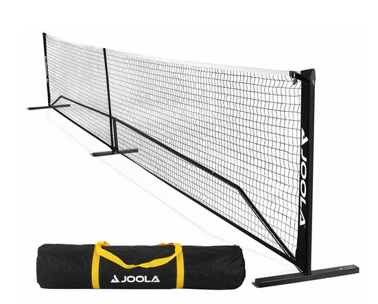
Mobiles Pickleball-Netz
Da gibt es übrigens auch kostengünstige Einsteigersets und Schläger mit einem guten Preis/Leistungsverhältnis und Mengenrabatten zu kaufen. Mit anderen Worten: Schulen und Sportvereine mit Zugang zu Badminton-Plätzen können mit wenig Aufwand und Kosten Pickleball anbieten! Und tatsächlich tun das immer mehr auch in Deutschland. Wir stehen meiner Meinung nach hierzulande vor einem Boom dieser Sportart.
Der Aufschlag im #Pickleball
Das Beste vorweg: Der Aufschlag im Pickleball ist leicht zu lernen und auszuführen. Anders als etwa im Tennis oder Tischtennis, wo man typischerweise viel Zeit mit der Übung des Aufschlags verbringt, um konkurrenzfähig zu sein. Die Regeln erschweren es zudem beträchtlich, dass der Aufschlag zur spielentscheidenden „Waffe“ werden kann. Asse oder zwingender Vorteil nach dem Aufschlag sind daher ziemlich selten.
RegelnDie Regeln zur Positionierung gelten sowohl für den Volley-Serve als auch für den Drop-Serve:
Zum Zeitpunkt, wenn der Ball beim Aufschlag auf den Schläger trifft, müssen die Füße des aufschlagenden Spielers hinter der Grundlinie und innerhalb verlängerten Linien der jeweiligen Platzhälfte sein:

Der Oberkörper des Spielers und der Ball dürfen sich dabei innerhalb des Spielfelds befinden. Außerdem darf der Spieler das Spielfeld betreten, unmittelbar nachdem der Ball den Schläger verlassen hat.
Vorher aber nicht:

Schon das Berühren der Grundlinie mit der Fußspitze beim Aufschlag ist ein Fehler.
Man darf auch nicht beliebig weit außen stehen:

Der linke Fuß ist hier außerhalb der verlängerten Linien der linken Platzhälfte, weshalb dieser Aufschlag nicht regelgerecht wäre.
Wer schlägt wann wohin auf, und was ist mit der NVZ?Es muss jeweils das diagonal gegenüberliegende Feld getroffen werden, wobei der Ball nicht in der NVZ landen darf. Die Linien gehören dabei zur NVZ: Ein Ball auf die hintere Linie der NVZ ist ein Fehler. Genauso gehören die Linien zum Aufschlagfeld: Ein Ball auf die Grundlinie oder ein Ball auf die Außenlinie ist also kein Fehler. Wird der Punkt gewonnen, wechselt der Aufschläger mit seinem Partner die Seite. Verliert der erste Aufschläger die Rally, macht sein Partner von der Seite weiter, wo er grad steht. Verliert auch der zweite Aufschläger die Rally, wechselt der Aufschlag auf das andere Team. Die Zählweise und die jeweilige Positionierung der Spieler hab ich in diesem Artikel behandelt.
Volley-ServeDas ist derzeit der beliebteste Aufschlag und ursprünglich auch der einzig erlaubte Aufschlag. Der Ball wird dabei aus der Hand aufgeschlagen.
Der Schlägerkopf muss dabei eine Bewegung von unten nach oben ausführen, wie in 4-3 zu sehen.
Der Schlägerkopf darf sich zum Zeitpunkt des Auftreffen des Balls nicht über dem Handgelenk befinden (4-1 zeigt die korrekte Ausführung, 4-2 ist ein häufig zu beobachtender Fehler).
Außerdem muss der Ball unterhalb der Taille des Aufschlägers getroffen werden, wie in 4-3 zu sehen.

Das obige Bild stammt aus dem Official Rulebook der USAP.
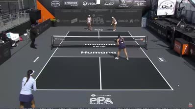
Alle Regeln zum Volley-Serve sollen im Grunde sicherstellen, dass dieser Aufschlag eben nicht zum spielentscheidenden Vorteil wird. Im folgenden Clip sehen wir einen Aufschlag von Anna Leigh Waters, der momentan besten Spielerin der Welt:
Diese Art des Aufschlags ist bei den Pros am häufigsten zu sehen: Volley-Serve, Top-Spin, tief ins Feld gespielt. Wir sehen aber auch, dass ihre Gegenspielerin den Aufschlag ohne große Mühe returniert. Asse oder direkt aus dem Aufschlag resultierender Punktgewinn sind im Pickleball ziemlich selten. Ganz im Gegensatz etwa zu Tennis und Tischtennis.
Drop-ServeDiese Art des Aufschlags ist erst seit 2021 erlaubt. Abgesehen von den oben beschriebenen Regeln zur Positionierung der Füße gibt es beim Drop-Serve nur eine weitere Regel: Der Ball muss aus der Hand fallengelassen werden. Hochwerfen oder nach unten Stoßen/Werfen des Balls ist nicht erlaubt. Insbesondere darf der Ball auf beliebige Art geschlagen werden. Das macht diesen Aufschlag besonders Einsteigerfreundlich, weil man kaum die Regeln verletzen kann.
Ich habe dem Drop-Serve bereits diesen Artikel gewidmet.
Abgesehen von den Regeln – wie sollte man aufschlagen?Es gibt hier zwei grundsätzliche Herangehensweisen:
Die einen sagen, weil man mit dem Aufschlag ohnehin selten einen direkten Punkt macht, sollte man ihn nur möglichst sicher in das hintere Drittel des Felds reinspielen:
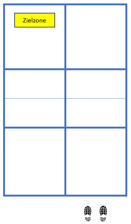
Ins hintere Drittel, weil die Rückschläger sonst zu leicht einen starken Return spielen und die Aufschläger hinten halten können. Mit der gelben Zielzone ist es unwahrscheinlich, dass der Aufschlag aus geht.
Die anderen (zu denen ich auch gehöre) sagen: Mit dem Aufschlag kann man ruhig etwas Risiko eingehen. Schließlich kann das Return-Team keinen Punkt machen. Es ist okay, wenn von 10 Aufschlägen 2 ausgehen und die übrigen 8 es den Rückschlägern schwer machen, uns hinten zu halten. Der eine oder andere direkte Punkt sollte auch dabei sein. Darum sehen meine Zielzonen so aus:
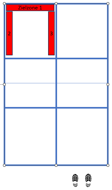
Die meisten Aufschläge gehen Richtung Zielzone 1, ab und an mal einer nach 2 und 3. Die roten Zonen sind deutlich näher an den Linien als die gelbe, was natürlich die Gefahr eines Ausballs erhöht.
Im Allgemeinen kann man zum Aufschlag im Pickleball sagen:
Länge ist wichtiger als Härte oder Spin. Ein entspannt in hohem Bogen ins hintere Drittel des Aufschlagfelds gelobbter Ball macht dem Rückschläger mehr Probleme als ein harter Topspin in die Mitte. Kurze Aufschläge sind sporadisch eingesetzt als Überraschungswaffe gut, ansonsten erleichtern sie es dem Rückschläger nur, nach vorn an die NVZ zu kommen.
Pickleball Übung: Drop Spiel 7-11
Einer der wichtigsten Schläge im Pickleball ist der 3rd Shot Drop – also der dritte Schlag einer Rally, wo das aufschlagende Team mittels eines kurzen Balls in die NVZ nach vorn kommen will.
Leider ist das auch ein ziemlich schwieriger Ball, weshalb er häufig geübt werden sollte.
Wenn es euch geht wie mir, findet ihr Spiele um Punkte viel spannender als Übungen. Darum hab ich mir dieses Spiel ausgedacht.
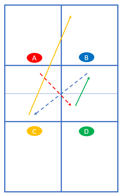
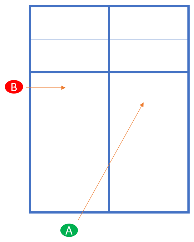
Es geht mit vier, drei oder sogar nur zwei Teilnehmern. Die Beschreibung ist für vier Spieler.
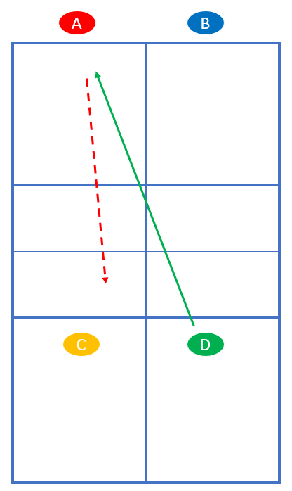
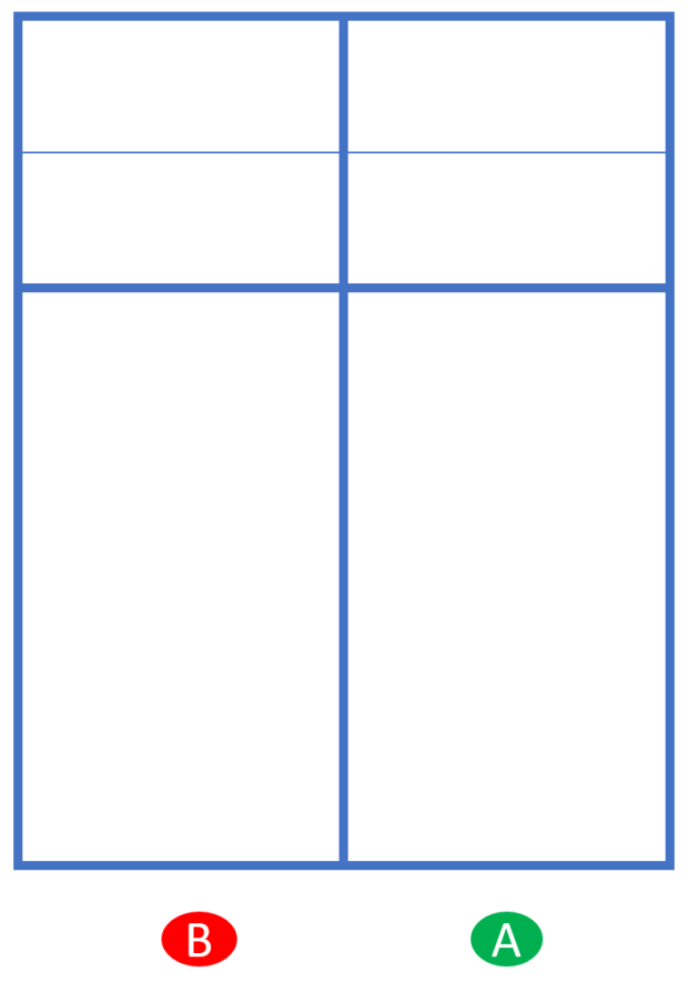
Spieler A und B sollen den Drop Shot üben. Sie stehen so, wie im normalen Spiel das aufschlagende Team vor dem 3. Schlag steht. Spieler C und D stehen so, wie im normalen Spiel das rückschlagende Team nach dem Return steht – nämlich an der NVZ. Hier in der Übung starten C und D jede Rally. Zuerst spielt D einen langen Ball diagonal. A versucht einen Drop Shot. Anschließend rücken A und B nach vorn:

Je nachdem, wie gut der Drop Shot war, kommen sie gleich nach vorn oder rücken allmählich durch die Transition-Zone vor.
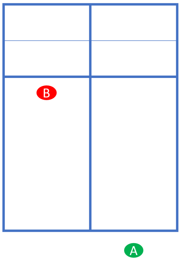
Das Spiel geht mit Rally-Scoring, also sowohl Team AB als auch Team CD können jederzeit Punkte machen. C und D starten abwechselnd die Rally. Ist also der erste Punkt ausgespielt, beginnt nun C:

Für C und D ist es etwas leichter, Punkte zu machen als für A und B. Darum gewinnen C und D mit 11 Punkten, während A und B schon mit 7 Punkten gewinnen.
Sind nur drei Spieler am Start, übt einer den Drop Shot. Er wechselt dabei jeweils die Seite. Die Gegner dürfen nur auf diese Seite spielen.
Bei zwei Spielern spielt man nur auf einer Hälfte des Platzes.
Das Spiel hat für beide Teams einen guten Übungseffekt, denn diese Schläge sind typischerweise die kritischen Schläge jedes Ballwechsels bei fortgeschrittenen Spielern – und man spielt/übt eben nur diese.
Durch das Scoring bleibt die Motivation hoch. Bei unseren bisherigen Drop Spielen hat sich gezeigt, dass nach relativ kurzer Zeit häufiger das Drop Team mit 7 Punkten gewinnt. Das ist aber auch ganz okay so, finde ich. Denn das gibt ja das Feedback, dass man es mit dem Drop Shot richtig macht.
1, 2, 3 – Frei!
Pickleball Übung: 1, 2 , 3 – Frei!
Eine schöne Übung zum Aufwärmen, die auch gut für Einsteiger geeignet ist:
Alle vier Spieler stehen an der NVZ. Aufschlag und Zählweise ist wie beim normalen Spiel.
Die ersten drei Bälle inklusive des Aufschlags müssen in der NVZ aufkommen. Anschließend ist der Ball freigegeben für offensive Dinks, Speed-Ups und Lobs:
Beispiel: Spieler A beginnt mit dem Aufschlag diagonal, D dinkt (nicht zwingend) zu B und B spielt den dritten Ball in die Küche zu C. C spielt einen langen Ball in die Lücke.
Hintergrund: Wir haben die Übung bisher so ähnlich gespielt, aber mit 5 Bällen, die in die Küche gespielt werden müssen, bevor der Ball freigegeben wird.
Das hat in meinen Augen zwei Nachteile:
- Es lehrt die Teilnehmer die falsche Art von Dinks, nämlich harmlose „Dead Dinks“ in die Küche. Im ernsthaften Spiel geht es aber beim Dinken nicht in erster Linie darum, unbedingt in die Küche zu treffen. Ein Dink soll möglichst nicht angreifbar sein, aber möglichst unangenehm für den Gegner, damit der einen hohen Ball zurückspielt, den wir unsererseits angreifen können. Das kann durchaus auch ein Ball sein, der kurz hinter der NVZ aufspringt. Mit dem alten Übungsmodell ist das aber ein Fehler. Später hat man dann oft noch Schwierigkeiten, den Leuten die richtige Art von Dinks beizubringen.
- Man muss bis 5 die Bälle mitzählen. Das klappt oft nicht so gut, so dass man im Zweifel ist: Waren das jetzt schon 5?
Bei 1, 2, 3 – Frei! behält man leichter den Überblick. Trotzdem ist der Aufschläger (wie beim großen Spiel) etwas im Nachteil, denn die Rückschläger können zuerst einen offensiven Ball spielen. Eben zum Beispiel einen druckvollen Dink, kurz hinter die NVZ.
Kompaktkurs Pickleball für Einsteiger

Alles was ihr braucht, um mit Pickleball qualifiziert zu starten. Auf den Punkt gebracht an einem Tag!
Dieser 4-stündige Kompaktkurs ist ideal geeignet für Berufstätige und sportlich ambitionierte Senioren.
Der Kurs kostet 40 Euro pro Person und wird geleitet von Uwe Hesse – einem erfahrenen Spieler und vom DPB zertifizierten Trainer.
Er findet statt in Düsseldorf.
Die Teilnehmerzahl ist je Kurs begrenzt auf 8, um ein intensives und individuelles Coaching gewährleisten zu können.
Inhalte sind u.a.
Grundschläge: Aufschlag, Return, Volley, Dink
Regelkunde
Basisstrategien im Doppel
Zählweise
Bedeutung der Non-Volley-Zone
3rd Shot Drop
Teilnehmer-Doppel mit Trainerfeedback
Aktuelle Termine:
Samstag, 27. April
Samstag, 04. Mai
Beginn ist jeweils 10:00 Uhr.
Anmeldungen bitte ausschließlich per Mail an info@uhesse.com
Für Mitglieder des DJK Agon 08 kostet der Kurs nur 20 Euro.
Bei nachfolgendem Vereinseintritt werden 20 Euro erstattet.
Pickleball Spaßturnier des DJK Agon 08
Der DJK Agon 08 hat erstmals ein Pickleball Spaßturnier durchgeführt. Das hat so gut geklappt und so viel Spaß gemacht, dass wir es sicher nächstes Jahr wiederholen werden!
19 Teilnehmer haben auf vier Plätzen gespielt – im Schnitt hat jeder 12 Spiele absolviert:
 Die vier Spielfelder auf unserer Clubanlage
Der Modus war denkbar einfach: Jeder sollte möglichst mit jedem gegen jeden spielen – ohne Rücksicht auf Alter, Spielstärke und Geschlecht. Das kann man im Pickleball gut machen, denn das Spiel ist ohnehin sehr inklusiv ausgelegt. So sind auch bei uns heute sehr viele schöne und auch ausgeglichene Spiele entstanden. Viele sind recht knapp entschieden worden.
Zwischendurch war auch fürs leibliche Wohl gesorgt worden:
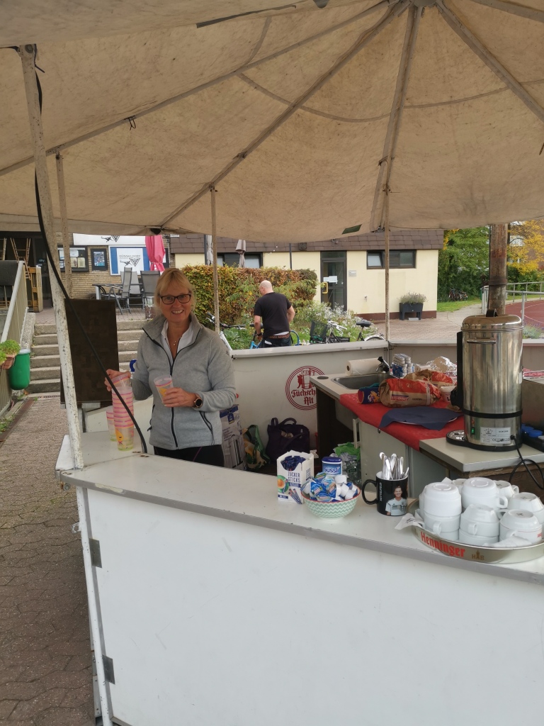 Danke nochmals an Beate & Christian für die Unterstützung, sowie für die Kuchenspenden auch von Elke, Susanne & Mitra!
Es gab auch Medaillen zu gewinnen:

Nach über vier Stunden Spielzeit stand der Sieger mit Fabio fest: Er hatte 42 Punkte aus 16 Spielen erzielt! Dicht gefolgt von Carsten mit 35 Punkten aus 15 Spielen:
 Carsten und Fabio mit den Medaillen, Uwe als Turnierleiter im Hintergrund
Michael hatte Bronze mit 34 Punkten aus 15 Spielen erreicht, war aber bei der Siegerehrung schon nicht mehr vor Ort.
Bei dem Turnier war auch ein gewisses Stehvermögen gefragt, denn wer wenig Pausen und viele Spiele machte hatte die besten Chancen auf die vorderen Plätze. Die Marke von 30 Punkten haben so hinter den drei ersten auch Andreas (30), Uwe (30), Annett (31) und Ross (33) geknackt!
Es hat uns bei diesem Turnier besonders gefreut, neben 7 DJK Mitgliedern auch 12 Teilnehmer aus anderen Vereinen begrüßen zu können.
Die Spiele waren jederzeit fair und freundlich, wie auch die gesamte Atmosphäre. Ich danke allen Teilnehmern herzlich für diese gemeinsame gelungene Aktion – das war erneut eine Werbung für unseren schönen Sport!
Stacking im Pickleball – Kurzer Leitfaden
Beim Doppel im Pickleball wird die Position der einzelnen Spieler (linke Seite oder rechte Seite) normalerweise durch den Spielstand bestimmt. Stacking ist eine Methode die Seite unabhängig vom Spielstand zu wählen. Der Begriff (Stacking = Stapelung) kommt daher, dass dabei häufig zwei Spieler vorübergehend auf derselben Seite stehen. Bisher sehe ich in meinem Umfeld kaum Stacking – auch bei den Deutschen Pickleball Meisterschaften 2022 habe ich es bei keinem Doppel beobachtet. Liegt wohl entweder daran, dass ich überwiegend bei Level 2.5 und 3.0 zugeschaut habe, oder daran, dass Pickleball in Deutschland ganz allgemein noch in den Kinderschuhen steckt, während Stacking eher eine Technik für Fortgeschrittene ist. Vielleicht wird es durch diesen Beitrag ja populärer.
Warum Stacking?Gründe für Stacking können sein
- Wir haben als Spieler im Team eine Lieblingsseite
- Linkshänder nach rechts
- Frau im Mixed nach rechts
- Stärkere Vorhand (bei Rechtshändern) nach links
- Die Gegner wollen immer einen von uns anspielen
- Als taktische Variante
Grundsätzlich ist es beim Pickleball im Doppel wichtig, sich die Ausgangspositionen zu merken: Wer anfangs rechts steht, wird zukünftig bei geradem Teamscore als Aufschläger und als Rückschläger rechts stehen müssen. Das gleiche gilt für den Spieler, der beim Stand von 0-0-2 links steht: Bei geradem Teamscore muss er jetzt und zukünftig als Aufschläger und als Rückschläger auf der linken Seite sein. Ein Verstoß gegen diese Regel führt streng genommen zum Verlust des Punkts bzw. der Ralley. Durch die beim Stacking erfolgenden Stellungswechsel ist die Gefahr etwas höher, da durcheinander zu kommen.
Stacking beim AufschlagWir betrachten zuerst Stacking beim Aufschlag. Das ist unsere Wunschposition:
Wir haben Aufschlag und stehen in Wunschposition bei 0-0-2: A links und B rechts. Unser Teamscore ist gerade: Alles ist wie sonst auch, kein Stacking nötig.
Wenn wir den Punkt gewinnen, steht es 1-0-2. Der Teamscore ist nun ungerade. Stacking passiert: A geht nur für den Aufschlag kurz nach links und wechselt dann wieder zurück nach rechts. B bleibt links:

Angenommen, im weiteren Spielverlauf verlieren wir das Aufschlagrecht, und es wechselt zu uns zurück beim Stand von 3-0-1. Unser Teamscore ist also ungerade. Bei ungeradem Score muss B rechts aufschlagen, daher erfolgt Stacking:

B geht nur für den Aufschlag kurz nach rechts und wechselt gleich danach wieder zurück auf die Lieblingsposition. A bleibt rechts stehen.
Zusammenfassung AufschlagBei geradem Teamscore schlagen wir wie üblich auf, jeder ist in Wunschposition.
Bei ungeradem Teamscore (1,3,5,7,9) passiert Stacking:
Der Aufschläger steht mittig nur für den Aufschlag auf der ungeliebten Seite, der Partner außen daneben.
Stacking beim ReturnAuch beim Return kann Stacking erfolgen. Bei geradem Teamscore haben wir ohnehin schon die Wunschposition und behalten die einfach bei, z.B. beim Stand von 3-2-1:
Bei ungeradem Teamscore passiert Stacking. Hier z.B. beim Stand von 3-1-1:

B muss den Return von der ungeliebten rechten Seite spielen. Er wird nach links wechseln und A nach rechts:

Angenommen, die Gegner machen den Punkt und servieren nun beim Stand von 4-1-1 von links. Zwar haben wir grad unsere Wunschposition (A rechts und B links) eingenommen, aber den Return von links muss beim Stand 4-1-1 zwingend A spielen. Also machen wir erneut Stacking:

Nach dem Aufschlag läuft A diagonal nach rechts an die NVZ, während B seitlich nach links wechselt.
VarianteAlternativ zum oben gezeigten Stacking kann der Partner auch schon direkt auf der bevorzugten Seite stehen:
Das macht unsere Absicht für den Gegner zwar offensichtlich, ist aber vielleicht etwas einfacher für uns in der Durchführung.
Zusammenfassung ReturnBeim Return erfolgt also Stacking ebenfalls bei ungeradem Team-score: Der Rückschläger läuft diagonal zur bevorzugten Seite an die NVZ und der Partner wechselt die Seite, bzw. steht schon auf seiner Lieblingsseite außen.
Flexibles StackingStacking kann auch nur von Fall zu Fall praktiziert werden. Mit Linkshändern im Team oder beim Mixed wird es häufig permanent während des ganzen Spiels gemacht. Flexibles Stacking kann benutzt werden, um dem Gegner das ständige Anspielen eines bestimmten Team-Mitglieds zu erschweren, oder als taktisches Mittel zwischendurch. Beim Aufschlag kann man sich absprechen und dann unmittelbar nach dem Service die Seiten wechseln. Beim Return kann der vorn stehende Partner Zeichen geben: Offene Hand hinter dem Rücken bedeutet: Ich wechsle die Seite. Der Rückschläger wird dann entsprechend diagonal auf die andere Seite laufen. Faust hinter dem Rücken bedeutet: Ich bleibe auf dieser Seite.
Stacking Pro & ContraSollte ich in meinen Doppelspielen Stacking einsetzen?
Pro
- Es ist nützlich bei Vorliebe für bestimmte Seite
- Man kann damit einen schwächeren Partner entlasten
- Es kann gut als taktisches Mittel eingesetzt werden
Contra
- Der Laufweg beim Return ist etwas länger
- Der Partner ist auch in Bewegung, was seinen Schlag etwas schwieriger macht
- Stacking erfordert ein eingespieltes Team
- Es wird für alle vier Spieler schwieriger, Spielstand und Spielerpositionen korrekt mitzuhalten
Die Punkte unter der Rubrik Contra sind der Grund, warum sich Stacking nur für fortgeschrittene, häufig zusammenspielende Doppel empfiehlt.
Das Video erläutert Stacking ähnlich wie der Artikel und zeigt auch als Beispiel, wie Profis Stacking praktizieren:
Pickleball 002 – Einstieg ins Doppel
Doppel ist sicherlich die beliebteste Variante in der Pickleball gespielt wird – viele spielen gar keine Einzel. Dieser kurze Artikel hilft vielleicht beim Einstieg. Das Beste vorweg: Pickleball im Doppel ist so ziemlich die inklusivste Form von Sport die man sich denken kann. Männer können gegen Frauen antreten, die ältere Generation gegen Jüngere, alte Hasen gegen Neueinsteiger. In praktisch jeder möglichen Kombination haben trotzdem alle ihren Spaß auf dem Feld und kommen auf ihre Kosten. Die Community ist gegenüber Neuankömmlingen sehr aufgeschlossen und wertschätzend. Das und die Inklusivität sind nach meiner Meinung auch die Hauptgründe, warum Pickleball so rapide an Popularität gewinnt.
Pickleball wird vorn entschiedenIm Tennis bin ich zwar eher ein Grundlinienspieler, aber das ist beim Pickleball nicht erfolgversprechend. Das kurze Spiel in der Nicht-Volley-Zone (NVZ) – auch Dinking genannt – und Volleys sind hier meistens spielentscheidend. Daher sollte man besonders Dinking und Volleys üben.
Üben für Ballsicherheit und KonsistenzÜbung macht den Pickleball-Meister, denn die meisten Spiele werden nicht so sehr gewonnen sondern durch unerzwungene Fehler verloren. Ballsicherheit ist Trumpf, natürlich auch und gerade im Doppel, wo man seinem Partner nicht gern viele unforced errors zumuten möchte. Eine gute Praxis ist es, vor dem eigentlichen Spiel zum Aufwärmen ein Kurz-Kurz-Spiel an der NVZ zu machen: Aufschlag diagonal, dann müssen erst mindestens 5 Dinks in die NVZ erfolgen, bevor der Ball freigegeben wird. Oder etwa, man muss erst 7 Volleys in Folge schaffen, bevor das Spiel anfängt.
Warum 0-0-2?Die Zählweise im Doppel kann anfangs verwirrend sein. Ich hab mich jedenfalls zunächst etwas schwer getan und darum dies Video aufgenommen:
Hilfreich ist es außerdem, wenn man sich im Doppel merkt, auf welcher Seite man am Anfang gestanden hat. Stehe ich zum Beispiel anfangs auf der rechten (geraden) Seite, so werde ich zukünftig immer, wenn mein Team einen geraden Punktestand hat, rechts stehen. Also bei 0,2,4,6,8,10 für mein Team sollte ich immer rechts stehen. Bei 1,3,5,7,9,11 sollte entsprechend mein Partner auf der linken (ungeraden) Seite stehen. Als Gedächtnisstütze nehme ich Schweißbänder: Zwei wenn ich rechts anfange und eines wenn ich links anfange.
Elementare Doppel-StrategieDie typische Verhaltensweise eines Doppel-Teams habe ich hier kurz geschildert. Natürlich gibt es noch mehr an Feinheiten, aber als Starthilfe sollte das erstmal reichen. Außerdem: So kompliziert ist Pickleball auch eigentlich nicht.
So, ich hoffe, das war hilfreich und ermutigend, um mit dem Pickleball spielen loszulegen – wir freuen uns schon darauf, euch auf dem Platz zu begegnen!
Impact of proper column precision for analytical queries
Does it matter if your data warehouse tables have columns with much higher precision than needed? Probably: Yes.
But how do you know the precision of your columns is larger than required by the values stored in these columns? In Exasol, we have introduced the function MIN_SCALE to find out. I’m working on an Exasol 7 New Features course at the moment, and this article is kind of a sneak preview.
If there’s an impact, it will show only with huge amounts of rows of course. Would be nice to have a table generator to give us large testing tables. Another Exasol 7 feature helps with that: The new clause VALUES BETWEEN.
CREATE OR REPLACE TABLE scaletest.t1 AS

SELECT CAST(1.123456789 AS DECIMAL(18,17)) AS testcol

FROM VALUES BETWEEN 1 AND 1e9;
This generates a table with 1000 million rows and takes only 30 seconds runtime on my modest VirtualBox VM. Obviously, the scale of the column is too large for the values stored there. But if it wouldn’t be that obvious, here’s how I can find out:
SELECT MAX(a) FROM (SELECT MIN_SCALE(testcol) As a FROM scaletest.t1);
This comes back with the output 9 after 20 seconds runtime, telling me that the precision actually required by the values is 9 at max. I’ll create a second table for comparison with only the required scale:
CREATE OR REPLACE TABLE scaletest.t2 AS

SELECT CAST(1.123456789 AS DECIMAL(10,9)) AS testcol

FROM VALUES BETWEEN 1 AND 1e9;
So does it really matter? Is there a runtime difference for analytical queries?
SELECT COUNT(*),MAX(testcol) FROM t1; -- 16 secs runtime
SELECT COUNT(*),MAX(testcol) FROM t2; -- 7 secs runtime
My little experiment shows, the query running on the column with appropriate scale is twice as fast than the one running on the too large scaled column!
It would be beneficial to adjust the column precision according to the scale the stored values actually need, in other words. With statements like this:
ALTER TABLE t1 MODIFY (testcol DECIMAL(10,9));
After that change, the runtime goes down to 7 seconds as well for the first statement.
I was curious if that effect shows also on other databases, so I prepared a similar test case for an Oracle database. Same tables but only 100 million rows. It takes just too long to export tables with 1000 million rows to Oracle, using VMs on my notebook. And don’t even think about trying to generate 1000 million row tables on Oracle with the CONNECT BY LEVEL method, that will just take forever – or more likely break with an out-of-memory error.
The effect shows also with 100 million row tables on Oracle: 5 seconds runtime with too large precision and about 3 seconds with the appropriately scaled column.
Conclusion: Yes, looks like it’s indeed sensible to format table columns according to the actual requirements of the values stored in them and it makes a difference, performancewise.
New free online course: #Exasol Virtual Schemas
Virtual Schemas integrate foreign data sources into the Exasol database. They enable Exasol to become the central source of truth in your data warehouse landscape.
We added another free online learning course to our curriculum that explains how to deal with Virtual Schemas. Like the others, it comes with many hands-on practices to support a good learning experience. It also contains many demo videos like this one:
I recorded this clip (like most of the others) myself, but this time we decided to do a voice-over by native professional speakers.
Certification exams are free, also for this new course. When you complete the majority of hands-on labs in the course, you get one free certification exam granted per person and per course.
What are you waiting for? Come and get it!
Eleven Table Tennis: Basics
Assuming you are an IRL player who wants to get as close to the real thing as possible, that’s what I’d recommend:
Make sure you have enough space to play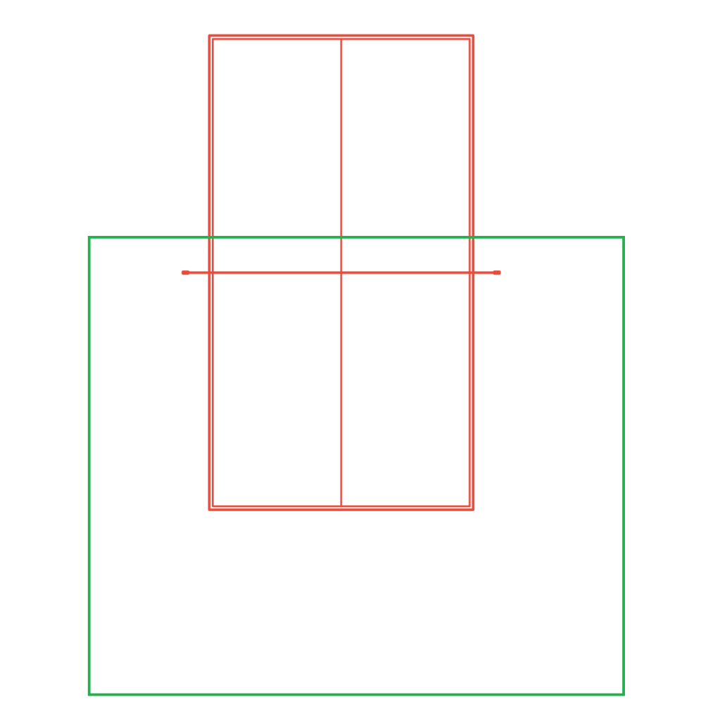
The green box is your playing space. It should be a square of 2.50 m X 2.50 m ideally. Make sure to leave some space at the front, so you can reach balls close to the net and even a little across the net. Otherwise you may become a victim of ghost serves. Leave enough room at the sides – some opponents play angled, just like IRL.
If you don’t have enough space for this setup – maybe you shouldn’t play multiplayer mode then. You can still have fun, playing against the ballmachine or against the AI. Actually, I think it’s worth the money even in that case.
Use the discord channelThe Eleven TT community is on this discord channel: https://discord.gg/s8EbXWG
I recommend you register there and use the same or a similar name as the name you have in the game. For example, I’m Uwe on discord and uwe. in the game (because the name uwe was already taken). This is handy to get advice from more experienced players, also the game developers are there. They are very responsive and keen to improve Eleven TT even more, according to your feedback.
There’s a preview version presently, that has improved tracking functionality. You can just ask the developers there to get you this preview version. I did, and I find it better than the regular version, especially for fast forehand strokes.
Setup your paddleWhen you have the Sanlaki paddle adapter (as recommended in the previous post), go to the menu and then to Paddle Settings:
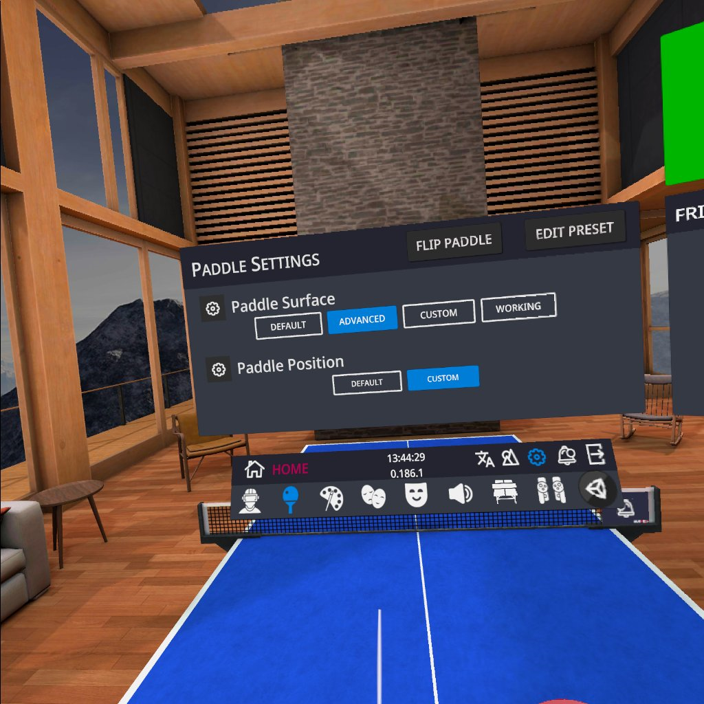
Click on Paddle Position and select the Sanlaki Adapter:

As an IRL player, you may start with an Advanced Paddle Surface:

Se how that works for you. Bounciness translates to the speed of your blade. An OFF ++ blade would be maximum bounciness. Spin is self-explaining. You have no tackiness attribute, though. Throw Coefficient translates to the sponge thickness. The higher that value, the thicker the sponge.
ServingThis takes some time to get used to. You need to press the trigger on the left controller to first “produce” a ball, then you throw it up and press the trigger again to release the ball. Took me a while to practice that and still sometimes I fail to release the ball as smoothly as I would like to.
What I like very much: You have a built-in arbiter, who makes sure your serve is legal according to the ITTF rules. That is applied for matches in multiplayer mode as well as for matches in single player mode. But not in free hit mode! Check out the Serve Practice:
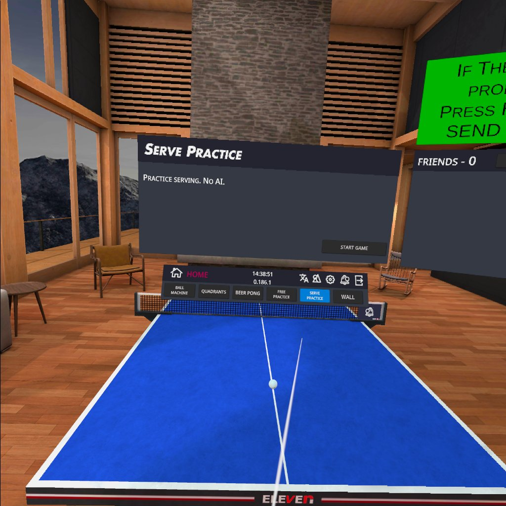
It tells you what went wrong in case:
 Remove AI Spin Lock

I recommend you practice with the AI opponent in single player mode for a while. It has spin lock on per default, which means it will never produce any side spin. I find that unrealistic. After some practicing against the AI in single player mode, you’re ready for matches in multiplayer mode against other human opponents.
BARC Survey confirms: #Exasol dominates Analytical Database Peers
Exasol leads the categories Performance, Platform Reliability and Support Quality for Analytical Database products. And we get a 100% recommendation score from the 782 customers in the survey.

So it’s not one of the big names in the industry who comes out on top of this survey. Not Oracle, not Teradata, not Snowflake, not SAP Hana leads in Analytical Databases but Exasol!
Customer quote: “Unbelievable query performance with almost zero administration effort. You just have to experience it yourself. Once you see it for yourself, you won’t want to work with any other database.”
To summarize:
- Exasol is the world’s fastest analytical database
- Exasol is reliable and easy to maintain
- Exasol’s services and attitude towards customers are highly appreciated
Compare that with your legacy platform: It’s time to contact us now!
How to enlarge an #Exasol database by adding a node
Adding a cluster node will not only increase the available storage capacity but also the total compute power of your cluster. This scale-out is a quite common operation for Exasol customers to do.
My example shows how to change an existing 2+1 cluster into a 3+0 cluster. Before you can enlarge the database with an active node, this node has to be a reserve node first. See here how to add a reserve to a 2+0 cluster. Of course you can add another reserve node to change from 3+0 to 3+1 afterwards. See here if you wonder why you may want to have a reserve node at all.
Initial state – reserve node is presentI start with a 2+1 cluster – 2 active nodes and 1 reserve node:
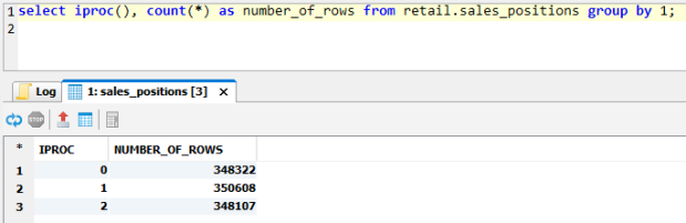
For later comparison, let’s look at the distribution of rows of one of my tables:

The rows are roughly even distributed across the two active nodes.
Before you continue, it would be a good idea to take a backup on a remote archive volume now – just in case.
Shutdown database before volume modificationA data volume used used by a database cannot be modified while that database is up, so shut it down first:
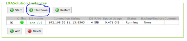
After going to the Storage branch in EXAoperation, click on the data volume:
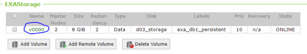
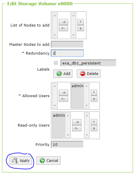
Then click on Edit:

Change the redundany from 2 to 1, then click Apply:

Why is the redundancy reduced from 2 to 1 here? Let’s try to explain that. Initially, I had 2 active nodes with a volume using redundancy 2:
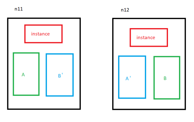
A and B are master segments while A’ and B’ are mirrored segments. If I could add a node to this volume keeping the existing segments, it would look like this:

Of course this would be a bad idea. The redundancy is reduced to 1 before the new node is added to the volume:

Only distributed master segments with no mirrors at first. Then the redundancy is again increased to 2:
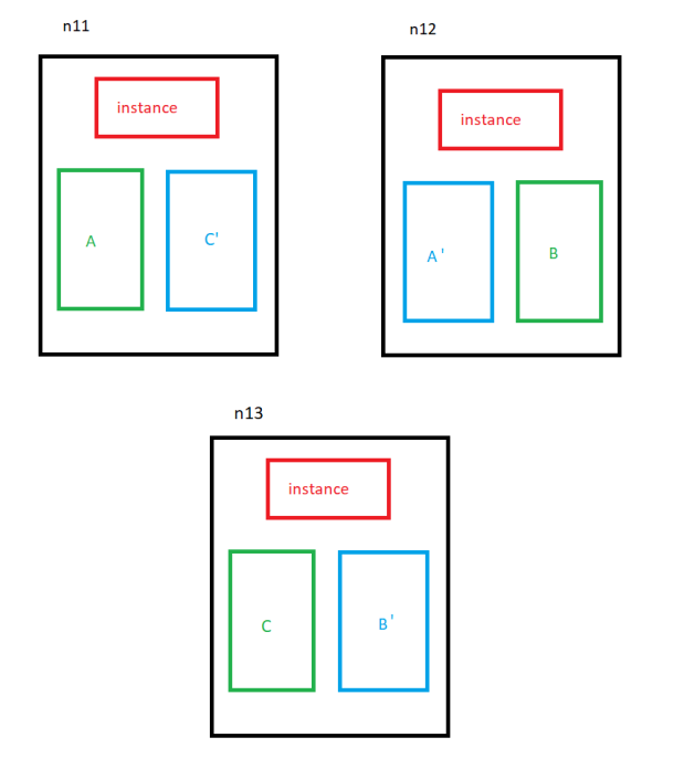
This way, every master segment can be mirrored on a neighbor node. That’s why the redundancy needs to be reduced to 1.
Add new node to volumeAfter having decreased the volume redundancy to 1, click Edit on the volume detail page again and add n13 as a new master node to the volume and click Apply:

Now click Edit again and increase the redudancy to 2:
The state of the volume shows now as RECOVERING – don’t worry, it just means that mirrored segments are now created.

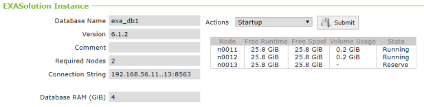
Now click on the database link on the EXASolution screen:

Select the Action Enlarge and click Submit:

Enter 1 and click Apply:

The database detail page looks like this now:

Technically, this is a 3+0 cluster now – but the third node doesn’t contain any data yet. If we look at the same table as before, we see that no rows are on the new node:
To change that, a REORGANIZE needs to be done. Either on the database layer, on schema layer or on table layer. Most easy to perform is REORGANIZE DATABASE:

Took me about 10 Minutes on my tiny database. That command re-distributes every table across all cluster nodes and can be time consuming with high data volume. While a table is reorganized, that table is locked against DML. You can monitor the ongoing reorganization by selecting from EXA_DBA_PROFILE_RUNNING in another session.
Final stateLet’s check the distribution of the previous table again:
As you can see above, now there are rows on the added node. Also EXAoperation confirms that the new node is not empty any more:

On a larger database, you would see that the volume usage of the nodes is less than before per node and every node is holding roughly the same amount of data. For failsafety, you could add another reserve node now.
Summary of steps- Add a reserve node (if not yet existing)
- Take a backup on a remote archive volume
- Shutdown database
- Decrease volume redundancy to 1
- Add former reserve node as new master node to the volume
- Increase redundancy to 2
- Enlarge database by 1 active node
- Reorganize
- Add another reserve node (optionally)
Getting started with Hyper-V on Windows 10
Microsoft Windows 10 comes with its own virtualization software called Hyper-V. Not for the Windows 10 Home edition, though.
Check if you fulfill the requirements by opening a CMD shell and typing in systeminfo:

The below part of the output from systeminfo should look like this:
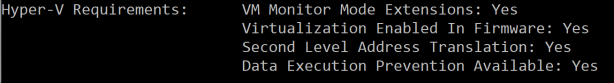
If you see No there instead, you need to enable virtualization in your BIOS settings.
Next you go to Programms and Features and click on Turn Windows features on or off:

You need Administrator rights for that. Then tick the checkbox for Hyper-V:

That requires a restart at the end:

Afterwards you can use the Hyper-V Manager:

Hyper-V can do similar things than VMware or VirtualBox. It doesn’t play well together with VirtualBox in my experience, though: VirtualBox VMs refused to start with errors like “VT-x is not available” after I installed Hyper-V. I also found it a bit trickier to handle than VirtualBox, but that’s maybe just because of me being less familiar with it.
The reason I use it now is because one of our customers who wants to do an Exasol Administration training cannot use VirtualBox – but Hyper-V is okay for them. And now it looks like that’s also an option. My testing so far shows that our educational cluster installation and management labs work also with Hyper-V.
Using DbVisualizer to work with #Oracle, #PostgreSQL and #Exasol
As a Database Developer or Database Administrator, it becomes increasingly unlikely that you will work with only one platform.
It’s quite useful to have one single tool to handle multiple different database platforms. And that’s exactly the ambition of DbVisualizer.
As a hypothecial scenario, let’s assume you are a database admin who works on a project to migrate from Oracle to EDB Postgres and Exasol.
The goal might be to replace the corporate Oracle database landscape, moving the OLTP part to EDB Postgres and the DWH / Analytics part to Exasol.
Instead of having to switch constantly between say SQL Developer, psql and EXAplus, a more efficient approach would be using DbVisualizer for all three.
I created one connection for each of the three databases here for my demo: Now let’s see if statements I do in Oracle also work in EDB Postgres and in Exasol:
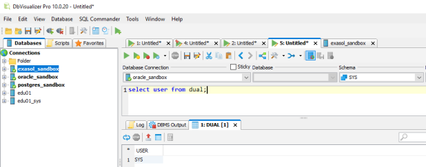
Oracle

EDB
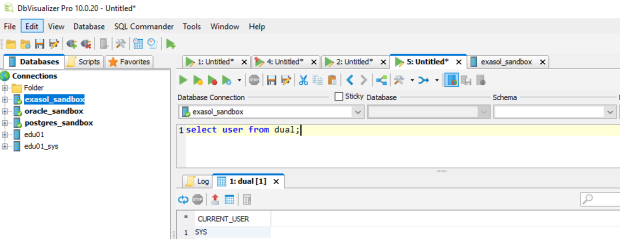
Exasol
Works the same for all three! The convenient thing here is that I just had to select the Database Connection from the pull down menu while leaving the statement as it is. No need to copy & paste even.
What about schemas and tables?
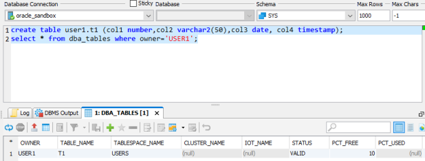
Oracle
In EDB, I need to create a schema accordingly:

EDB
In Exasol, schema and table can be created in the same way:

Exasol
Notice that the data types got silently translated into the proper Exasol data types:
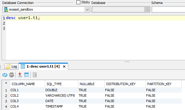
Exasol
There is no DBA_TABLES in Exasol, though:
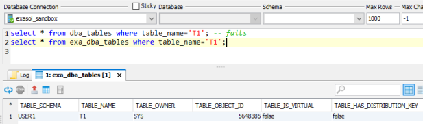
Exasol
Of course, there’s much more to check and test upon migration, but I think you got an idea how a universal SQL Client like DbVisualizer might help for such purposes.
Comparison between #Oracle and #Exasol
After having worked with both databases for quite some time, this is what I consider to be the key differences between Oracle and Exasol. Of course the two have much in common: Both are relational databases with a transaction management system that supports the ACID model and both follow the ANSI SQL standard – both with some enhancements. Coming from Oracle as I do, much in Exasol looks quite familiar. But let’s focus on the differences:
StrengthsOracle is leading technology for Online Transaction Processing (OLTP). If you have a high data volume with many users doing concurrent changes, this is where Oracle shines particularly.
Exasol is leading technology for analytical workloads. If you want to do real-time ad hoc reporting on high data volume, this is where Exasol shines particularly.
Architecture Data Format & In-Memory processingOracle uses a row-oriented data format, which is well suited for OLTP but not so much for analytical workloads. That’s why Hybrid Columnar Compression (only available on Engineered Systems respectively on Oracle proprietary storage) and the In-Memory Column Store (extra charged option) have been added in recent years.
Exasol uses natively a compressed columnar data format and processes this format in memory. That is very good for analytical queries but bad for OLTP because one session that does DML on a table locks that table against DML from other sessions. Read Consistent SELECT is possible for these other sessions, though.
Oracle was designed for OLTP at times when memory was scarce and expensive. Exasol was designed to process analytical workloads in memory.
ClusteringOracle started as a non-clustered (single instance) system. Real Application Clusters (RAC) have been added much later. The majority of Oracle installations is still non-clustered. RAC (extra charged option) is rather an exception than the rule. Most RAC installations are 2-node clusters with availability as the prime reason, scalability being rather a side aspect.
Exasol was designed from the start to run on clustered commodity Intel servers. Prime reasons were MPP performance and scalability with availability being rather a side aspect.
Data DistributionThis doesn’t matter for most Oracle installations, only for RAC. Here, Oracle uses a shared disk architecture while Exasol uses a shared nothing architecture, which is optimal for performance because every Exasol cluster node can operate on a different part of the data in parallel. Drawback is that after adding nodes to an Exasol cluster, the data has to be re-distributed.
With Exadata, Oracle tries to compensate the performance disadvantage of the shared disk architecture by enabling the storage servers to filter data locally for analytical workloads. This approach leads to better performance than Oracle can deliver on other (non-proprietary) platforms.
Availability & RecoverabilityClearly, Oracle is better in this area. A non-clustered Oracle database running in archive log mode will enable you to recover every single committed transaction you did since you took the last backup. With Exasol, you can only restore the last backup and all changes since then are lost. You can safeguard an Oracle database against site failure with a standby database at large distance without performance impact. Exasol doesn’t have that. With RAC, you can protect an Oracle database against node failure. The database stays up (the Global Resource Directory is frozen for a couple of seconds, though) upon node failure with no data loss.
If an Exasol cluster node fails, this leads to a database restart. Means no availability for a couple of seconds and all sessions get disconnected. But also no data loss. Optionally, Exasol can be configured as Synchronous Dual Data Center – similar to Oracle’s Extended RAC.
Complexity & ManageabilityI realized that there’s a big difference between Exasol and Oracle in this area when I was teaching an Exasol Admin class recently: Some seasoned Oracle DBAs in the audience kept asking questions like “We can do this and that in Oracle, how does that work with Exasol?” (e.g. creating Materialized Views or Bitmap Indexes or an extra Keep Cache) and my answer was always like “We don’t need that with Exasol to get good performance”.
Let’s face it, an Oracle database is probably one of the most complex commercial software products ever developed. You need years of experience to administer an Oracle database with confidence. See this recent Oracle Database Administration manual to get an impression. It has 1690 pages! And that’s not yet Real Application Clusters, which is additionally 492 pages. Over 2100 pages of documentation to dig through, and after having worked with Oracle for over 20 years, I can proudly say that I actually know most of it.
In comparison, Exasol is very easy to use and to manage, because the system takes care of itself largely. Which is why our Admin class can have a duration of only two days and attendees feel empowered to manage Exasol afterwards.
That was intentionally so from the start: Exasol customers are not supposed to study the database for years (or pay someone who did) in order to get great performance. Oracle realized that being complex and difficult to manage is an obstacle and came out with the Autonomous Database – but that is only available in the proprietary Oracle Cloud.
PerformanceUsing comparable hardware and processing the same (analytical) workload, Exasol outperforms any competitor. That includes Oracle on Exadata. Our Presales consultants regard Exadata as a sitting duck, waiting to get shot on a POC. I was personally shocked to learn that, after drinking the Oracle Kool-Aid myself for years.
In my opinion, these two points are most important: Exasol is faster and at the same time much easier to manage! I mean anything useless could be easy to manage, so that’s not an asset on its own. But together with delivering striking performance, that’s really a big deal.
LicensingThis is and has always been a painpoint for Oracle customers: The licensing of an Oracle database is so complex and fine granular that you always wonder “Am I allowed to do this without violating my license? Do we really need these features that we paid for? Are we safe if Oracle does a License Audit?” With Exasol, all features are always included and the two most popular license types are totally easy to understand: You pay either for the data volume loaded into the cluster or for the amount of memory assigned to the database. No sleepless nights because of that!
CloudThis topic becomes increasingly important as many of our new customers want to deploy Exasol in the cloud. And you may have noticed that Oracle pushes going cloud seriously over the last years.
Exasol runs with all features enabled in the cloud: You can choose between Amazon Web Services, (AWS), Microsoft Azure and ExaCloud
AWSThis is presently the most popular way our customers run Exasol in the cloud. See here for more details.
MS AzureMicrosoft’s cloud can also be used to run Exasol, which gives you the option to choose between two major public cloud platforms. See here for more details.
ExaCloudHosted and managed by Exasol, ExaCloud is a full database-as-a-service offering. See here for more details.
Hybrid Exasol deployments that combine cloud with on-prem can also be used, just depending on customer requirements.
Oracle offers RAC only on the Oracle Cloud platform, not on public clouds. Various other features are also restricted to be available only in Oracle’s own cloud. The licensing model has been tweaked to favor the usage of Oracle’s own cloud over other public clouds generally.
Customer ExperienceCustomers love Exasol, as the recent Dresner report confirms. We get a perfect recommendation score. I can also tell that from personal encounters: Literally every customer I met is pleased with our product and our services!
ConclusionOracle is great for OLTP and okay for analytical workloads – especially if you pay extra for things like Partitioning, RAC, In-Memory Column Store and Exadata. Then the performance you get for your analytical workload might suit your present demand.
Exasol is totally bad for OLTP but best in the world for analytical workloads. Do you think your data volume and your analytic demands will grow?
Recover dropped tables with Virtual Access Restore in #Exasol
The technique to recover only certain objects from an ordinary backup is called Virtual Access Restore. Means you create a database from backup that contains only the minimum elements needed to access the objects you request. This database is then removed afterwards.
Let’s see an example. This is my initial setup:
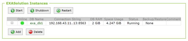
One database in a 2+1 cluster. Yes it’s tiny because it lives on my notebook in VirtualBox. See here how you can get that too.
It uses the data volume v0000 and I took a backup into the archive volume v0002 already.

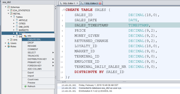
I have a schema named RETAIL there with the table SALES:
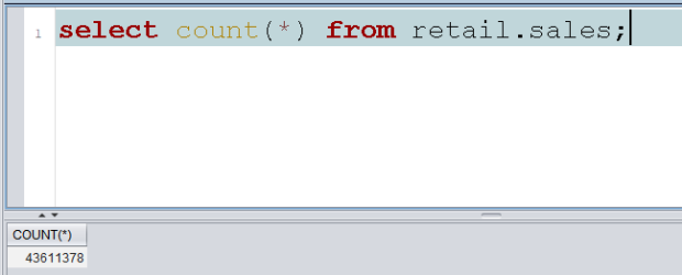
By mistake, that table gets dropped:

And I’m on AUTOCOMMIT, otherwise this could be rolled back in Exasol. Virtual Access Restore to the rescue!
First I need another data volume:

Notice the size of the new volume: It is smaller than the overall size of the backup respectively the size of the “production database”! I did that to prove that space is not much of a concern here.
Then I add a second database to the cluster that uses that volume. The connection port (8564) must be different from the port used by the first database and the DB RAM in total must not exceed the licensed size, which is limited to 4 GB RAM in my case:

I did not start that database because for the restore procedure it has to be down anyway. Clicking on the DB Name and then on the Backups button gets me here:

No backup shown yet because I didn’t take any backups with exa_db2. Clicking on Show foreign database backups:
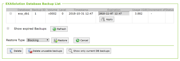
The Expiration date must be empty for a Virtual Access Restore, so I just remove it and click Apply. Then I select the Restore Type as Virtual Access and click Restore:

This will automatically start the second database:

I connect to exa_db2 with EXAplus, where the Schema Browser gives me the DDL for the table SALES:
I take that to exa_db1 and run it there, which gives me the table back but empty. Next I create a connection from exa_db1 to exa_db2 and import the table
create connection exa_db2
to '192.168.43.11..13:8564'
user 'sys' identified by 'exasol';

import into retail.sales
from exa at exa_db2
table retail.sales;
This took about 2 Minutes:

The second database and then the second data volume can now be dropped. Problem solved!
Understanding Partitioning in #Exasol
Exasol introduced Partitioning in version 6.1. This feature helps to improve the performance of statements accessing large tables. As an example, let’s take these two tables:

Say t2 is too large to fit in memory and may get partitioned therefore.
In contrast to distribution, partitioning should be done on columns that are used for filtering:
ALTER TABLE t2 PARTITION BY WhereCol;
Now without taking distribution into account (on a one-node cluster), the table t2 looks like this:

Notice that partitioning changes the way the table is physically ordered on disk.
A statement like
SELECT * FROM t2 WHERE WhereCol=’A’;
would have to load only the red part of the table into memory. This may show benefits on a one-node cluster as well as on multi-node clusters. On a multi-node cluster, a large table like t2 is distributed across the active nodes. It can additionally be partitioned also. Should the two tables reside on a three-node cluster with distribution on the JoinCol columns and the table t2 partitioned on the WhereCol column, they look like this:

That way, each node has to load a smaller portion of the table into memory if statements are executed that filter on the WhereCol column while joins on the JoinCol column are still local joins.
EXA_(USER|ALL|DBA)_TABLES shows both the distribution key and the partition key if any.
Notice that Exasol will automatically create an appropriate number of partitions – you don’t have to specify that.
Accelerate your #BI Performance with #Exasol
Your BI users complain about slow performance of their analytical queries? Is this your Status Quo?

tableau was taken as a popular example for AdHoc analytics but it might be any of the others like MicroStrategy, Looker, you name it. The good news is that this problem can be solved quite easily and without having to spend a fortune trying to speed up your legacy DWH to keep up with the BI demands:

Using Exasol as a High Performance Sidecar to take away the pain from your BI users is the easy and fast cure for your problem! This is actually the most common way how Exasol arrives at companies. More often than not this may lead to a complete replacement of the legacy DWH by Exasol:

That’s what adidas, Otto and Zalando did, to name a few of our customers.
Don’t take our word for it, we are more than happy to do a PoC!